Chapter 8. Parallel Vector Algorithms
8.1 Introduction
Next, we study several algorithms where parallelism can be easily expressed in terms of array operations. We will use Fortran 90 to represent these algorithms.
Simplistic timing figures will be given in some cases for pipelined machines and array machines.
In these timings, subscript computations and memory access/communications costs will be ignored.
8.2 Target machines
The natural target machines for programs with vector parallelism are array machines and pipelined processors.
It is also easy to exploit vector parallelism on shared memory multiprocessors and on message-passing multicomputers. However, the best parallel form for these machines sometimes cannot be expressed in vector notation.
8.3 Time to execute a vector operation
Let us start with the simplest possible situation. Consider the following generic vector operation:
a(1:n) # b(1:n)
First, let us assume a pipelined arithmetic unit with s# stages for operation #. Each stage takes t units of time.
The time to execute the vector operation under these assumptions is :
Compare this with the serial time when no pipelining takes place:
Consider now an array machine with P arithmetic units.
The execution time is:
where t# is the time to execute one # operation.
In a system where each processing unit contains an arithmentic pipeline, the execution time would be:
8.4 Reductions in Fortran 90
A typical reduction is
sum(array)
which returns,as we should expect, the sum of the elements of an integer, real, or complex array. It returns zero if
array
has size zero.
Others include:
all(mask)
Returns the logical value .true. if all elements of of the logical array
mask
are
.true.
or
mask
has size zero, and otherwise returns the value
.false.
any(mask)
Returns the logical value
.true.
if any of the elements of the logical array
mask
is
.true.
, and returns the value
.false.
if no elements are
.true.
or if
mask
has size zero.
count(mask)
Returns the number of
.true.
values in
mask.
maxval(array)
Returns the maximum value of the elements of an integer or real array.
minval(array)
Returns the minimum value of the elements of an integer or real array.
product(array)
returns the product of the elements of an integer, real, or complex array. It returns 1 if
array
has size zero.
All these functions have an optional argument
dim
if this is present, the operation is applied to all rank-one sections that span right through dimension
dim
to produce an array of rank reduced by one and extends equal to the extents in the other dimensions. For example, if
a
is a real array of shape [4,5,6],
sum(a,dim=2)
is a real array of shape [4,6] and element (i,j) has value
sum(a(i,:,j)).
The functions
maxval
,
minval
,
product
, and
sum
have a third optional argument,
mask
. If this is present, it must have the same shape as the first argument and the operation is applied to the elements corresponding to true elements of
mask
; for esample,
sum(a,mask=a>0)
sums the positive elements of the array
a
.
8.5 Two other useful Fortran 90 functions.
1. spread(source,dim,ncopies)
Returns an array of rhe same type as
source
but with rank increased by one over
source
.
Source
may be a scalar or an array.
Dim
and
ncopies
are integer scalars. The result contains
max(ncopies,0)
copies of source, and element (r1,...,rn+1) of the result is source (s1,...,sn) where (s1,...,sn) is (r1,...,rn+1) with subscript
dim
omitted (or
source
itself if it is a scalar).
Example of use:
a=spread(x,dim=2,ncopies=n)+spread(x,1,n)
w=sum(abs(a),dim=1)
is equivalent to:
do i=1,n
w(i)=0
do j=1,n
w(i)=w(i)+abs(x(i)+x(j))
end do
end do
2. maxloc(array[,mask])
Returns a rank-one integer array of size equal to the rank of
array.
Its value is the subscript of an element of maximum value.
8.6 Time to Execute a Reduction
Consider a reduction such as:
r = sum(a(1:n)) = a(1) + a(2) + a(3) + ... a(n)
or, in general
r = a(1) # a(2) # a(3) # ... a(n)
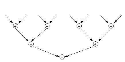
A sequence of Èlog2n vector operations of length n/2, n/4, ..., 1 suffices to compute the reduction (assuming associativity of the # operation).
Therefore (assuming n=2m):
An alternative way of performing a reduction, which was implemented in the Cray-1, proceeded by feeding the pipeline elements of the vector to be reduced together with the output of the pipeline. Thus, in the case of
sum
, the elements of the input vector are added to the output of the pipeline as shown in the figure below. The pipeline is assumed to produce the identity of the reduction operation (zero in the case of a sum) until the first element of the vector exits the pipe.
At the end of the process, there will be s# (the number of stages used by the pipe to perform the # operation) partial results which should be added to get the final result. The time to get the final result is therefore:
In the case of an array machine, there are two cases. First, if P < n/2, and if we follow the approach presented in our discussion of reductions in OpenMP, we have:
If the final reduction can also be done in logarithmic time using a reduction tree approach:
In this case, the execution time is:
If P >= n/2, the time is:
The # operation could be a simple arithmetic operation such as s + or * or it could be a more complex binary operation. For example, to implement
maxloc
in logarithmic time we could define an operation
on two pairs consisting of a value and a location:
(v1,loc1) # (v2,loc2)=
if v1 < v2 then return (v1,loc1)
else return (v2,loc2)
And, to implement an in logarithmic time an operation that finds the location of the first negative value in a vector we could define the following similar operation:
(v1,loc1) # (v2,loc2)=
if v1 < 0 then return (v1,loc1)
else return (v2,loc2)
Notice that both of these operations are associative (but NOT commutative).
8.7 Parallel Prefix
Consider the following loop:
			A(0)=0
			DO I=1,N
				A(I)=A(I-1)+B(I)
			END DO
The loop seems sequential because each iteration needs information on the value computed in the preceding iteration.
However, we can use a parallel prefix approach to compute the value of vector A in parallel as follows:
A parallel program implementing this strategy under the assumption that N=2k is:
	A(1:N)=B(1:N)
	DO	I=0,K-1
		A(2**I+1:N)=A(2**I+1:N)+A(1:N-2**I+1)
	END DO
For an array machine with the number of procesing units P>=n-1:
As in the case of reduction, parallel prefix can be applied to any associative binary operation.
8.8 Relative Performance
How much faster does a program run when executed in parallel?
Speedup: SP=T'1/ TP (1)
T'1: Execution time of the program on a single (scalar) processor.
TP: Execution time on a parallel machine.
Parallel programs may introduce some redundancy to achieve higher parallelism. In a sequential program, the goal is to minimize the total number of operations because this number is directly related to the execution time. In a parallel program, this relationship is not direct. For this reason a more honest formula for speedup is:
Speedup: SP=T1/ TP (2)
where T1 is the best known serial version of the program.
The speedup in (1) is known as the parallel speedup.
Assume a multiprocessor with P processors or an array machine with P processing elements. The speedup can be linear in P (that is, of the form k*P for k <= 1), logarithmic (that is, of the form k * log P), or it can have many other forms. In a real machine the speedup is seldom a nice function of the number of processors.
In some cases the speedup is superlinear; that is, the speedup is greater than p for p processors. This happens when, for example, each processor has its own cache memory. In this way using several processors also increases the size of the cache memory. Another case when you can get superlinar speedup is in program performing some form of search operation.
Other important measures include:
where P is the number of processors if the target machine is a multiprocessor (assuming single-user mode) or the number of processing elements in an array processor.
where OP is the number of operations in the parallel program, and O1 is the number of operations in the best known serial version.
8.9 Examples of Speedup and Efficiency
Consider
a(1:n) + b(1:n)
The speedup, efficiency, and redundancy on a pipelined unit are:
In an array machine:
The value of SP is P if n is a multiple of P.
EP is 1 if n is a multiple of P. Otherwise it is < 1.
The speedup, efficiency, and redundancy of the parallel prefix example on an array machine with P=n are:
8.10 Amdahl's Law
Assume a program which executes in one of two modes: serial or perfectly parallel. In the perfectly parallel mode, as many processors as desired can cooperate in the execution of the program. Assume that s is the fraction of the program that is serial and q is the fraction that is parallel. The speedup of this program, given p processors is then
SP = T ( s + q ) / T(s + q / P) = 1 / (s + q /P)
When P is large, the speedup curve is very steep near s = 0. To obtain a very high speedup, the serial fraction of the program has to be very small.
The form of this curve has been used to argue that is difficult to obtain good speedups. However, there are many examples where good speedups are obtained (see Gustafson: Reevaluating Amdahl's law. CACM Vol 31, No. 5. pp. 532-533). The argument is that the problem size tends to grow with the number of processors. If this is the case, we have:
Scaled speedup = (s + q * P)/(s+(q*P)/P) = P + (1-P) * s
This is a line with a moderate slope.
8.11 Matrix-Vector Multiplication
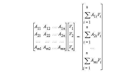
In mathematical notation:
In Fortran:
do i=1,m
R(i) = 0
do j=1,n
R(i) = R(i) + A(i,j) * V(j)
end do
end do
The inner loop performs a dot product (or inner product) of two vectors. It can be represetned in Fortran 90 as follows:
do i=1,m
R(i)=DOT_PRODUCT(A(i,1:n),V(1:n))
end do
The dot product is a vector multiplication (of length n, in this case) followed by a reduction.
Time in a pipelined machine for a dot product:
The total time for the matrix-vector multiplication is then:
In an array machine or in a multiprocessor, the time if P>n is:
Alternatively, by interchanging the loop headers, the program could be written as follows:
do j=1,n
do i=1,m
R(i) = R(i) + A(i,j) * V(j)
end do
end do
This leads to the following sequence of vector operations:
do j=1,n
R(1:m)=R(1:m)+A(1:m,j)*V(j)
end do
The time for this loop in a pipelined machine is:
if there is no chaining, and
if there is chaining.
Assume two consecutive vector operations where the second operation uses the output from the first. Chaining allows the two operations to behave as if there were a single pipeline for both operations. This is achieved by feeding the output from the pipeline executing the first operation directly to the second pipeline. The alternative is to wait for the first opeation to complete before starting the second operation.
To illustrate chaining. consider the two statements:
a(1:n)=b(1:n)*c(1:n)
e(1:n)=a(1:n)+d(1:n)
Ignoring memory accesses and subscript computations, and assuming 4 stages for multiplication and 3 for addition, we have the following time lines in the absence of chaning:
But, in the presence of chaning, the time lines would look as follows:
In an array machine or in a multiprocessor, the time (if P > m) is:
8.12 Matrix Multiplication
do i=1,n
do j=1,n
do k=1,n
C(i,j)=C(i,j)+A(i,k)*B(k,j)
end do
end do
end do
do i=1,n
do j=1,n
C(i,j)=DOT_PRODUCT(A(i,1:n),B(1:n,j))
end do
end do
The time on a pipelined machine is:
The time on an array machine or multiprocessor if P > n is:
do j=1,n
do k=1,n
do i=1,n
C(i,j)=C(i,j)+A(i,k)*B(k,j)
end do
end do
end do
do j=1,n
do k=1,n
C(1:n,j)=C(1:n,j)+A(1:n,k)*B(k,j)
end do
end do
Alternatively, the headers could have been exchanged in a different order to obtain the loop:
do i=1,n
do k=1,n
C(i,1:n)=C(i,1:n)+A(i,k)*B(k,1:n)
end do
end do
The time on a pipelined machine, assuming chaining, is:
The time in an array machine is:
-
Outer-product method (n2-parallelism)
Another interchange of the loop headers produce:
do k=1,n
do i=1,n
do j=1,n
C(i,j)=C(i,j)+A(i,k)*B(k,j)
end do
end do
end do
To obtain n2 parallelism, the inner two loops should take the form of a matrix operation:
do k=1,n
C(1:n,1:n)=C(1:n,1:n)+A(1:n,k) B(k,1:n)
end do
Where the operator
represents the outer product of two vectors. Given two vectors a and b, their outer product is a matrix Z such that Zi,j=ai
¥
bj . Notice that the previous loop is NOT a valid Fortran or Fortran 90 loop because
is not a valid Fortran character.
The outer product matrix in the loop above has the following form:
This matrix is the element-by-element product of the following two matrices:
which are formed by replicating
Ak
=
A(1:n,k)
and Bk=
B(k,1:n)
along the appropriate dimensions. This replication can be achieved using the Fortran 90
SPREAD
function discussed above:
spread(A(1:n,k),dim=2,ncopies=n)*spread(B(k,1:n),dim=1,ncopies=n))
The resulting loop is therefore:
do k=1,n
C=C+SPREAD(A(1:n,k),2,n)*SPREAD(B(k,1:N,1,n)
end do
In an array machine with P>n2, the time would be:
where tcopy is the time to copy a vector. The time to
spread
to n copies is logarithmic as discussed in class.
The product of two n
¥
n matrices,
C=matmul(A,B)
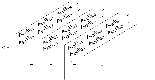
, can be computed by adding n matrices of rank (n,n):
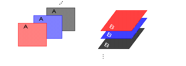
These n matrices of rank (n,n) can be computed by multiplying (element-by-element) two three-dimensional arrays of rank(n,n,n).
The two three-dimensional arrays are formed by replicating A and B along different dimensions as shown next:
This replication can, again, be achieved, with
SPREAD
.
Thus, give the following three directions of replication:
we can start by computing a n3 temporary array T as follows:
T(:,:,:)=SPREAD(A,DIM=3,NCOPIES=n)*SPREAD(B,DIM=1,NCOPIES=n)
Then, the result is just
C=SUM(T,DIM=2)
In an array machine with P>=n3 processing unit, the time to compute C would be:
8.13 Multiplication by Diagonals
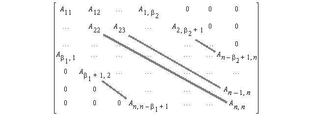
An n
¥
n matrix A is banded if Aij=0 for i-j
b
1, j-i
b
2:
For a small band, for example,
b
1=
b
2=3, the algorithm discussed before for matrix-vector multiplication is not efficient.
An alternative is to do the product by diagonals:
After separating the diagonals into separate matrices, we get:
which can be written as follows:
where Vj=(Vj,...,Vn) and Vn-j=(V1,...,Vn-j).
Also,
means add the sorter vector to the first component of the longer one, and
/
means add the shorter vector to the last component of the longer one.
In Fortran 90 (except for the greek letters and the subscripts):
A0(1:n)*V(1:n) +
(/ A1(1:n-1)*V(2:n),0. /) +
...
(/  Ab
1(1:n-b
1)*V(b
1+1:n), (0., j=1,b
1) /) +
(/ 0., A-1(1:n-1)*V(1:n-1) /) +
...
(/ (0., j=1,b
2), Ab
2(1:n-b
2)*V(1:n-b
2) /)
8.14 Consistent Algorithms
A vector algorithm for solving a problem of size n is consistent with the best serial algorithms for the same problem if the redundancy is bounded as n
Æ
·.
Vector reduction is consistent.
But parallel prefix is not (see Section 8.9).
The time for the simple form of parallel prefix presented in Section 8.7 given P processing units and vector length n=2k is:
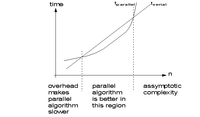
The problem with algorithms that are non consistant is that for n (size of input data) large enough, the array algorithm is slower than the scalar version. Assuming constant number of devices (pipeline stages or processing units).
For example, assuming 8 processors tparallel has the following values:
|
n
|
tserial
|
tparallel
|
|
16
|
15
|
7
|
|
32
|
31
|
17
|
|
64
|
63
|
41
|
|
512
|
511
|
513
|
|
1024
|
1023
|
1153
|
|
~106
|
~106
|
~2.5
¥
106
|
Notice that the array algorithm becomes slower than the scalar version when n=512.
A typical situation with inconsistent algorithms is depicted in the following graph:
8.15 A consistent version of parallel prefix
A consistent version of parallel prefix can be obtained by blocking the original algorithm. This can be done for both a pipelined unit or an array machine. We will show the array machine version. There are several steps in the algorithm
-
First the array B(1:n) should be reshaped into an
 matrix as follows:
C=RESHAPE(B,(/  , P /),0.0)
The
reshape(source,shape[,pad][,order])
function takes the elements of
source
, in normal Fortran order, and returns them (as many as will fit) as an array whose shape is specified by the one-dimensional integer array
shape
. If there is space remaining, then
pad
must be specifie and is used to fill out the rest. See the manual for a description of
order
.
Thus, if
B = (/1.,2.,3.,4.,5.,6.,7.,8.,9.,10.,11. /)
then, the result of
RESHAPE
above would be:
-
Then, we assign a column of
C
to each processing unit and compute the partial sums of each column separately as follows:
do i=2, 
C(i,1:P) = C(i-1,1:P) + C(i,1:P)
end do
-
The third step is to compute the true value of the last element of each column:
do j=2,P
			C( ,j)= C(
 ,j-1)+C(
 ,j)
,j)
end do
At the end of this step, the last element of each column will have the sum of all elements in its own column and the columns preceding it.
-
Finally, the elements in each processor are adjusted:
do i=1,  -1
-1
C(i,2:P) = C(  ,1:P-1) + C(i,2:P)
end do
The total number of operation in the algorithm is:
The algorithms is consistent because:
8.16 Cyclic Reduction
Let
One way to solve the recurrence in parallel is to use cyclic reduction:
From
and
we get
Which can be rewritten as
where ai(1) and bi(1) are defined as follows:
Now we have Si as a function of Si-2.
If we repeat this process several times we obtain
where
Initially,
When the subscript of ai, bi or Si is outside the range 1,...,n, the value 0 should be assumed
When l = log n
To compute the a's and b's in parallel we proceed as shown below
The resulting program in Fortran 90 is
S(1:n)=b(1:n)
do i=1,logn
S(1:n)=EOSHIFT(S(1:n),-2**(i-1))*a(1:n)+S(1:n)
a(1:n)=EOSHIFT(a(1:n),-2**(i-1))*a(1:n)
end do
The function
eoshift(array,shift [,boundary] [,dim])
returns the result of end-off left-shifting every one-dimensional section of
array
(in dimension
dim
) by
shift
. If
shift
is negative, the array is shifted to the right. If
boundary
is present as a scalar, it supplies the elements to fill in the blanks; if it is not present, zero is used. If
dim
is not present, one is assumed.
8.17 The
FORALL
statement
"One of the positive effectns of Fortran 90's long gestation period has been the general recognition, both by the X3J3 committee and by the community at large, that Fortran needs to evlove over time. Fortran 95 is a minor, but by no means insginificant, updating of Fortran 90."
It includes
PURE
and
ELEMENTAL
procedures, the
DIM
argument for
maxloc
and
minloc
, and the
FORALL
statement.
"Because the inside iteration of a
FORALL
block can be done in any order, or in parallel, there is a logical difficulty in allowing functions or subroutines inside such blocks: If the function or subroutine has side effects
(that is, if it changes any data elsewhere in the machine, or in its own saved variables) then the result of a
FORALL
calculation could depend on the order in which the iterations happen to be done. This can't be tolerated, of course; hence a new
PURE
attribute for subprograms."
The
FORALL
statement is used to specify an array assignment in terms of individual elements or sections.
For example,
A(1:10,2:20)=5*B(2:11,1:19)
can al be written as follows:
forall(i=1:10,j=1:19)A(i,j+1=5*B(i+1,j)
Notice that
FORALL
specifies a vector operations and therefore, the right-hand side is evaluated before any part of the left-hand side is changed.
Thus, the previous assignment can be written as:
do i=1,10
do j=1,19
A(i,j+1)=5*B(i+1,j)
end do
end do
because the right and left-hand sidesare disjoint, but
forall (j=1:n) A(j)=5*A(j-1)
should be written as two loops:
do j=1,n
temp(j)=5*A(j-1)
end do
do j=1,n
A(j)=temp(j)
end do
A singlle loop would not do in this case.
Notice that sometimes a single loop would suffice even if there is overlap betwenn left- and right-hand sides. Thus,
forall (j=1:n) A(j)=5*A(j+1)
Is equivalento to the loop:
do j=1,n
A(j)=5*A(j=1)
end do
Several examples of
FORALL
are presented next:
1. FORALL(I=1:10) A(I,I)=B(I,I)
can be written as
A(1:10)=B(1:10)
or as
A=B
if both
A
and
B
have shape
(10)
.
2. FORALL(I=1:10:2,J=10:1:-1)A(I,J)=B(I,J)*C(I,J)
can be written as
A(1:10:2,10:1:-1)=B(1:10:2,10:1:-1)*C(1:10:2,10:1:-1)
3. FORALL(I=1:10)A(I)=I
Is equivalent to
A(1:10)=(/1:10/)
4. FORALL(I=1:10,J=1:20)A(I,J)=B(I)
Needs SPREAD
 to be implemented because array sections in an assignment statement have to be comformable.
A=SPREAD(B,DIM=2,NCOPIES=20).
5. FORALL(I=1:10,J=1:10)A(I,J)=B(J,I)
Can be implemented with the
TRANSPOSE
intrinsic functions.
6. FORALL(I=1:N) A(I,I)=B(I,I)
or the slightly more complex statement:
FORALL(I=1:N) A(I,I)=B(I+1,I-1)
would need
RESHAPE
(or
EQUIVALENCE
) to be written as vector operations is Fortran 90. Thus, the first
FORALL
could be written as:
T1(1:N*N)=RESHAPE(B,(\N*N\))
T2(1:N*N)=RESHAPE(A,(\N*N\))
T2(1:N*N:N+1)=T1(1:N*N:N+1)
A=RESHAPE(T2,(\N,N\))
The second
FORALL
is left as an excercise.
7. FORALL(I=1:N,J=1:N,K=1:N,
& I+J+K.EQ.3*(N+1)/2)
& A(I+J-K,J)=B(I,J,K)
This statement includes a boolean expression. Only for those elements where the expression is true, an assignment will take place.
8.
	FORALL(I=1:10,J=1:20,K=1:30)
& A(I,J,K)=I+J+K
For this statement
SPREAD
is needed:
A=SPREAD(SPREAD((/1:10/),2,20),3,30)
& +SPREAD(SPREAD((/1:20/),1,10),3,30)
& +SPREAD(SPREAD(/1:30/),1,10),2,20)
9. FORALL(I=2:2000)A(I)=A(I/2)
This pattern is a standard technique for representing a binary tree structure as an array; the two children of of element k are elements 2k and 2k+1. This statment causes every node in the tree to receive a copy of information from its parent; it might be part of a computation that pipelines data down the leaves of the tree in a breadth-first fashion.
10. FORALL(I=1:10,J=1:10,K=1:10)
& A(I,J,K)=B(J,K,I)
This particularly simple example, can be expressed with the
RESHAPE
intrinsic, which provides for permuting axes while reshaping.
11. FORALL(I=1:10,J=1:10,K=1:10)
& A(I,J,K) = B(J,11-K,I+1)
In this case one would have to use
RESHAPE
to transpose the axes and then use an array section assignment to do the rest of the job. This would be relatively inefficent, resulting in multiple copying of data.
8.18 Sorting in Fortran 90.
There are many parallel sorting algorithms. We will discuss two very simple ones in this chapter and more elaborate algorithms later in the semester.
Perhaps the simplest sorting algorithm is bubble sort. (Text extracterd from Kumar et al. Introduction to Parallel Computing) It compares and exchages adjacent elements in the sequence to be sorted. Given the sequence a1, a2, ...,an, the algorith first performs n-1 compare-exchange operations in the following order: (a1,a2),(a2,a3), ...(an-1,an). This step moves the largest element to the end of the sequence. The last ement in the sequence is then ignored, and the sequence of compare exchanges is applied to the resulting sequence. The sequence is sorted after n-1 iterations. The algorithm is as follows:
do i=n-1,1,-1
do j=1,i
if (a(j) > a(j+1) ) swap (a(j),a(j+1))
end do
end do
Where
swap(a,b)
is just the sequence
t=a
a=b
b=t
This algorithm can be easily parallelized as discussed later on.
For vectorization, we will use the following slightly modifed version known as odd-even transposition:
do i=1,n
	if i
 is odd
 then
do j=0,n/2-1
if (a(2*j+1)>a(2*j+2)) swap(a(2*j+1),a(2*j+2))
end do
end if
	if i
 is even
 then
do j=1,n/2-1
if (a(2*j)>a(2*j+1)) swap(a(2*j),a(2*j+1))
end do
end if
end do
The algorithm alternates between two phases: odd and even. During the odd phase, elements with odd indices are compared with their right neighbors, and if they are out of sequence they are exchanged. Similarly, during the even phase, elements with even indices are compared with their right neighbors, and if they are out of sequence they are exchanged.
Vectorization is quite simple:
do i=1,n
if i is odd then
where (a(1:n-1:2)>a(2:n:2))
swap (a(1:n-1:2),a(2:n:2))
end where
end if
if i is even then
where (a(2:n-2:2)>a(3:n-1:2))
swap (a(2:n-2:2),a(3:n-1:2))
end where
end if
end do
Bubble sort is not a very efficient algorithm. It takes n(n-1)/2 comparisons to complete. The parallel version reduces that to n steps, but a good sequential algorithm only requires a number of comparisons proportional to n log n. And there are paralle algorithm that require time proportional to log2n. So this is ok, but not great.
A better sorting algorithms in some situations is radix sort. This was the algorithm used to sort punched cards with electro-mechanical devices.
The idea is that the values to be sorted are assumed to be numbers in a certain radix. Integers could be radix 10 or 2 depending on the circumstances. For punched cards, it was base 10. In today's machines, we could assume base two, but any other base can be assumed. When values are names, base 26 can be assumed.
Radix sort, goes through all the "digits" starting with the less significant one. For each digit it processes the whole sequence. Elements of the sequence are placed in separate buckets, one for each possible digit. Placement in the buckets is in the order theelements appear in the sequence. After processing all elements for a particular position, the buckets are catenated to create the sequence for the next position.
Consider for example the following sequence:
223, 148, 221, 071, 138, 131.
After the first step, the sequence will be separated as follows:
bucket 0 1 2 3 4 5 6 7 8 9
221 223 148
071 138
131
After catenation, we get: 221,071,131,223,148,138.
Now, the digits in the second position are processed:
bucket 0 1 2 3 4 5 6 7 8 9
221 131 148 071
223 138
Again,the buckets are catenated: 221,223,131,138, 148,071.
Then, the digits in the third position are processed:
bucket 0 1 2 3 4 5 6 7 8 9
071 131 221
138 223
148
Finally, the sorted sequence is obtained by catenating the buckets: 071,131,138,148, 221, 223.
The algorithm can be easily implemented in Fortran 90 using the
pack
intrinsic function.
Pack(array, mask)
returns a one-dimensional array containing the elements of
array
to pass the
mask
.
Thus, assuming that the sequence to be sorted is in vector
a
, and that the elements are in base b and contain d digits each, we can proceed as follows:
do i=1,d
	m_0(1:n) = the digit in
a(1:n)
 with weight bi-1 is 0
	m_1(1:n) = the digit in
a(1:n)
 with weight bi-1 is 1
...
	m_b1(1:n) = the digit in
a(1:n)
 with weight bi-1 is b-1
a=(/pack(a,m_0),pack(a,m_1),...,pack(a,m_b1)/)
end do
In particular for base 2, only one mask is needed:
do i=1,d
m=mod(a,2**i)<2**(i-1)
a= (/pack(a,m),pack(a,.not.m)/)
end do
Pack can be implemented in parallel using the primitives discussed earlier in class:
function pack(a,m)
where (m)
c=1
elsewhere
c=0
end where
order=parallel_prefix(c)
where (m)
temp(order)=a
end where
pack=temp
return
end
8.19 Processing linked lists
Lined lists are usually represented with pointer. Pointer values are usually memory addresses. However, linked lists can also be represented using array locations.
For example, a linked list could be represented using two arrays. One containing the
value
of the list entry, and the other conaining the position within the array where the
next
element in the list is located.
Now, a vector algorithm to make vector
next
point to the last entry in the list is as follows
:
do while (any(next/=null).and.any(next(next)/=null))
where(next(next)/=null)
next=next(next)
end where
end do
And a vector algorithm to do parallel prefix computation in the order of the linked list is as follows:
do while (any(next /= null))
where (next /= null)
value(next)=value+value(next)
next=next(next)
end where
end do
8.20 The Wavefront method (a.k.a. the Hyperplane method)
In this chapter we will only consider a simple two dimensional Fortran 77 form of this method. That is, we will only consider two dimensional loop nests with a single statement inside that assigns to a two dimensional array.
To illustrate this method we will draw a graph of the iteration space of the loop. Each iteration will be a node in the graph. The graph will taked the form of a mesh with equal vertical and horizontal separation.
These nodes will be joined by three classes of arcs representing races (write-read, read-write, write-write). These arcs (which are called dependences) will always flow in the direction of execution in the original loop.
The idea is that a vector form can be obtained by finding a collection of parallel lines that are equidistant, are not parallel to any dependence arc, and pass through all the nodes in the graph.
For example, the loop
do i=1,n
do j=1,n
a(i,j)=a(i-1,j)+1
end do
end do
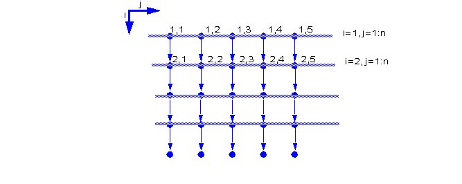
can be represented by the following graph:
From the graph it is clear that for each i there is a vector operation in j.
do i=1,n
a(i,1:n)=a(i-1,1:n)+1
end do
A second example:
do i=1,n
do j=1,n
a(i,j)=a(i,j-1)+a(i+1,j+1)+b(i)+c(j)
end do
end do
Now for each j there is a vector operation
do j=1,n
a(1:n,j)=a(1:n,j-1)+a(2:n+1,j+1)+b(i)+c(1:n)
end do
A more complicated case:
do i=2,n
do j=2,n
a(i,j)=a(i,j-1)+a(i-1,j)
end do
end do
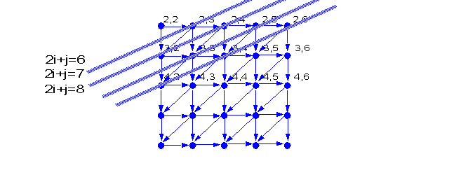
From the equations:
We conclude that:
From where:
do k=4,2*n
forall (i=max(2,k-n):min(n,k-2)) a(i,k-j)=...
end do
Another complex example:
do i=2,n
do j=2,n
a(i,j)=a(i+1,j-1)+a(i-1,j)+a(i,j-1)
end do
end do
From the equations:
We conclude that:
From where:
do k=6,3*n
forall (i=max(2,(k-n+1)/2):min(n,(k-2)/2)) a(i,k-j)=...
end do










 matrix as follows:
 , P /),0.0)


 ,j)= C(
 ,j-1)+C(
 ,j)
,j)
 -1
-1
 ,1:P-1) + C(i,2:P)


